Why Opening Statistics Are Wrong

When we choose which opening moves to play, many of us take opening statistics seriously into consideration, often more so than computer evaluations or master-level theory. This is reasonable: a +0.8 advantage on move 5 matters little when every other move in the middlegame is a blunder. Computer and master moves may be the best in theory, but are not necessarily the ones that provide the best practical chances for amateur blitz players.

So, we dive into the opening explorer, choose our rating range and look for moves that offer a high win rate at our level. This is not the only criterion of course (simplicity and soundness matter a lot to me), but it is an important one. Whether an amateur should even bother with all that is a different question but whatever floats our boats.

The problem with opening statistics is that they are wrong. By “wrong”, I do not mean of course that there is some error in the code that calculates them. I mean that the methodology of grouping by *average* rating is flawed. If you are a 2100-rated player and choose the “2000-2200” category in the opening explorer, you want to see how people with your rating perform when they play different openings. Instead, you get a substantially distorted picture of that. That is because you get the statistics on games where the *average* rating of the two players is in the [2000,2200) range (greater or equal to 2000, smaller than 2200).

I have no way to explain this without a small numerical example, so allow me some time to construct a very simple hypothetical with assumptions that may at first appear a bit outrageous, but will allow us to see things more clearly. One could show the same thing mathematically in a more rigorous way, but who’s got time for that?

Assume that:
A) We have only four players (A, B, C, D) with white colors, their ratings being respectively 1950, 2050, 2150 and 2250.
B) The 1950-rated player (A) plays 100 games against unnamed 1850-rated players, 100 games against 1950-rated players, and 100 games against 2050-rated players.
C) And so on for the other 3 players with the white color... Each of them plays a total of 300 games, distributed equally across lower rated, equally rated, and higher rated opponents.
D) Our 2 first players with ratings of 1950 and 2050 (A and B) play the opening move “X”, while the other 2 players with ratings of 2150 and 2250 (C and D) play the opening move “Y”. It is well documented that players of different strengths play different openings. My example here is extreme, but I want to make a point in the simplest way possible.
E) Both openings (X and Y) are practically speaking equally good. Of course the openings played by higher-rated players tend to be better in real life. Otherwise they wouldn’t play different openings! Trust me, though, that making opening “Y” slightly better will not alter the conclusion of our story.
F) A player will score a 75% win rate against those rated 100 points below, a 50% win rate against equals, a 25% win rate against better players. These numbers are the same for opening X and Y, per assumption E. There are no draws.

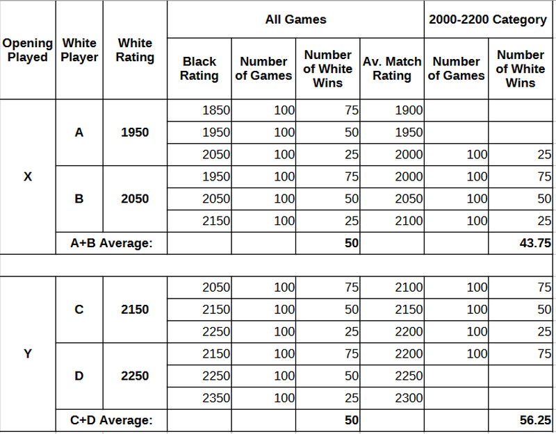
The following table lists all four white players, and the games they play against their opponents, and the results of their games:

For example, we see that the 2050-rated player B plays 100 games against 1950-rated opponents and scores 75% against them. Similarly, player B plays 100 games against 2150-rated opponents and scores 25% against them, etc.

In the right part of the table, we see only those games that are counted when calculating average opening statistics for the 2000-2200 rating range. (In the Opening Explorer, this range does not include matches with an average of exactly 2200, but this is irrelevant as we could have simply subtracted some ε>0 from the rating of player D, and the example would work exactly the same way).

The moral of the story:
I) The true average win rate for both openings is 50% -- this is by construction, a direct outcome of our assumptions, so nothing new here.
II) The win rates reported under the 2000-2200 average rating category turn out to be 43.75% for opening X and 56.25% for opening Y. So, if you saw this in the Opening Explorer, you would conclude that opening Y is superior to X, while they are exactly the same (by construction).

The culprit behind this statistical illusion is nothing but the grouping by average rating. This sort of grouping inflates the win rate of opening Y compared to X, because of an asymmetry: We have in our sample 100 games played by the 1950-rated player A against 2050-rated opponents, where he scores only 25%. On the opposite end of the spectrum, we have 100 games played by the 2250-rated player D against 2150-rated opponents, where he scores 75%. So the inclusion of these two “guests” in our sample, players A and D, distorts opening statistics.

If I made the example a bit more complicated, another distortion in the same direction would be visible: The sample does *not* include games where 2000-something white players beat 1900-something players by playing X. It also misses games where almost-2200 players lose to 2300-rated black players, by playing Y. Adding all that would strengthen the statistical illusion of a difference in the practical chances offered by the two openings.

There are two questions to address now: is this important enough in practice? If so, can it be fixed? I’ll answer the two questions in reverse order.

The fix: Instead of grouping the games based on the average rating of both players, we should group by the rating of white players if we want to see things from white’s point of view. Similarly, we should group by the rating of players with black, if we want to see things from their point of view. Think of this like the personal statistics tab in the Opening Explorer, where you get to choose between your games with white and your games with black. In the example above, if we construct the “2000-2200” white category by aggregating all the games of B and C (and nothing more), we can easily see that both X and Y come with a win rate of 50%, equal to the assumed truth.

Is this easy to implement? Probably yes, but I am out of my depth here, the code of Opening Explorer is incomprehensible to me.

So, what’s going on in the actual data?

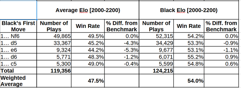
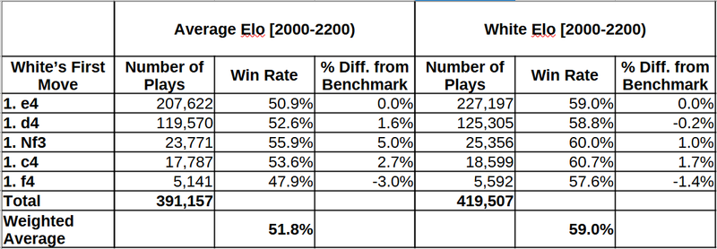
The table below reports the win rates (calculated as % Win + 0.5 * % Draw) for the first move played in blitz games in January 2017 (2000-2200 category). I used the January 2017 sample from the Lichess database, because it would take too much time and computing resources to analyze a large dataset with what I have. I hope I will soon repeat this with larger samples.

I present only the first five most common moves, because the standard errors get bigger further below and getting into discussions of statistical significance is beyond the point in this article. In this part of the table, standard errors are small enough for us to not worry much about them. I take the win rate of 1.e4 as the benchmark to compare the win rates of the other moves. The first half of the table uses the categorization of the Opening Explorer, by the average rating of the match. The second half uses the methodology I propose: categorizing by the rating of players of the relevant color.

What we see is that the success rates of different opening moves are much closer together when I use the proposed methodology. While it appears that 1. Nf3 outperforms 1. e4 by 5% in the traditional 2000-2200 grouping, this advantage drops to only 1% when using the grouping by white rating only. So, if you were considering 1. Nf3 because of the practical chances it offers, you should just choose whichever move you like. Quite interestingly, 1. f4 is only half as bad as it looks! I rarely play this move, but I always believed in it! Keep in mind these are numbers from years ago, so the current picture may look different.

The total number of games includes all first moves, even those not presented in detail. The weighted average of win rates for white goes substantially up with the proposed methodology. This is because the new methodology gets rid of the type-A and type-D “guests”. Note that the type-A “guests” are more common than type-D, since there are more 1900+ rated players than 2200+ players. To put it simply, the games of 1900+ rated white players are gone (and that’s good!).

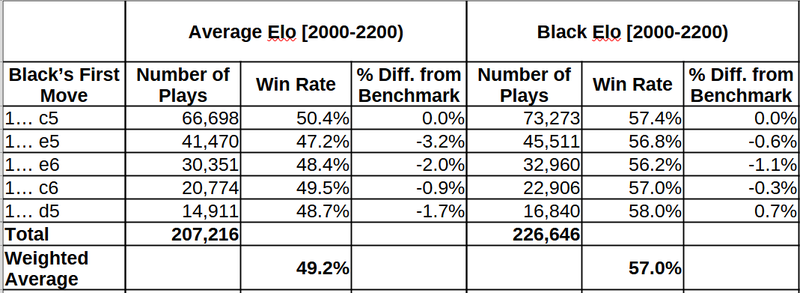
Next, we have the top-5 responses to 1.e4, using the win rate of black in the Sicilian (1... c5) as our benchmark.

Again, the top-5 moves seem a lot closer together when I use the proposed methodology. The distance between 1... e5 and 1... c5 is gone, and the Scandinavian looks suddenly very appealing (not statistically significant, though, so I’d wait to see the results with larger and more recent samples). It may seems surprising that we have a 57% win rate for black, but keep in mind that a) this is below the 59% win rate for white in the 2000-2200 range, and b) generally win rates go up for both colors as rating increases and this is a range quite far up there (not as much as I’d like to, lol).

Finally, we get to the question that inspired this: What to play against 1.d4?

The first part of the table, shows that 1... Nf6 (the benchmark) and 1... c5 are better than 1... d5, and 1...e6, and slightly better than 1...d6. The second part, though, shows that all these moves are actually much more similar in their win rates than they appear at first.

All the above results suggest one thing: disregard opening statistics and choose sound openings that you enjoy (what your tutor told you anyway). The differences in the actual win rates are very small, though often statistically significant. It is possible that the application of this methodology in larger datasets may reveal interesting differences in win rates in some positions. However, I suspect that within the subset of sound moves, deviations in win rates will be generally smaller than they appear now. I may come back with more material in the future, if there is interest.

I look forward to any comments, suggestions, corrections!

Big thanks to the Lichess Team for all that they provide, and to David J. Barnes, creator of pgn-extract, without which there would be no way for me to run this data analysis.

*UPDATE*
After the discussion in the comments, I did the same analysis again, but this time I added a restriction on the difference between the ratings of the two players that they should be less than 100. I barely thought about implementing this when I first wrote the post because:
a) I didn't expect too many games to be played between players of very different ratings (wrong!)
b) I was interested in the results of 2000-2200 players against the full range of their opponents. However, if that is the case we should find a way to deflate wins against much lower opponents. There are some interesting ideas in the comments, but I'll work on that later.
c) My intuition was that the results would not be affected by much. The results below suggest that I was half-right: there is some impact, but the main result remains the same: grouping by the average rating of both players tends to exaggerate differences in the win rates of various first moves, while grouping by white (black) rating to study the statistics for white's moves (black's moves) is much better. Various other problems with opening statistics remain, as discussed also in the comments.

Overall, I conclude that some sort of a restriction in the rating difference helps to keep the noise out, or alternatively some method of deflation is needed. Below are the updated results:

Black's responses against 1.e4:

Black's responses against 1.d4: